Wiki Contributions
Comments
Hmm maybe I'm misunderstanding something, but I think the reason I'm disagreeing is that the losses being compared are wrt a different distribution (the ground truth actual next token) so I don't think comparing two comparisons between two distributions is equivalent to comparing the two distributions directly.
Eg, I think for these to be the same it would need to be the case that something along the lines
or
were true, but I don't think either of those are true. To connect that to this specific case, have be the data distribution, and and the model with and without replaced activations
Reconstruction score
on a separate note that could also be a crux,
measures how replacing activations changes the total loss of the model
quite underspecifies what "reconstruction score" is. So I'll give a brief explanation:
let:
- be the CE loss of the model unperturbed on the data distribution
- be the CE loss of the model when activations are replaced with the reconstructed activations
- be the CE loss of the model when activations are replaced with the zero vector
then
so, this has the property that when the value is 0 the SAE is as bad as replacement with zeros and when it's 1 the SAE is not degrading performance at all
It's not clear that normalizing with makes a ton of sense, but since it's an emerging domain it's not fully clear what metrics to use and this one is pretty standard/common. I'd prefer if bits/nats lost were the norm, but I haven't ever seen someone use that.
I think these aren't equivalent? KL divergence between the original model's outputs and the outputs of the patched model is different than reconstruction loss. Reconstruction loss is the CE loss of the patched model. And CE loss is essentially the KL divergence of the prediction with the correct next token, as opposed to with the probability distribution of the original model.
Also reconstruction loss/score is in my experience the more standard metric here, though both can say something useful.
I want to mention that in my experience a factor of 2 difference in L0 makes a pretty huge difference in reconstruction score/L2 norm. IMO ideally you should compare pareto curves for each architecture or get two datapoints that have almost the exact same L0 if you want to compare two architectures.
I agree with pretty much all these points. This problem has motivated some work I have been doing and has been pretty relevant to think well about and test so I made some toy models of the situation.
This is a minimal proof of concept example I had lying around, and insufficient to prove this will happen in larger model, but definitely shows that composite features are a possible outcome and validates what you're saying:
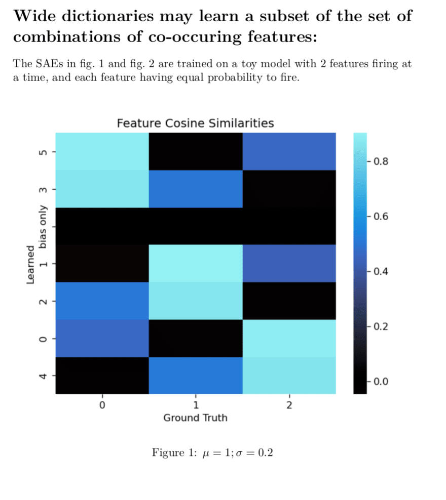
Here, it has not learned a single atomic feature.
All the true features are orthogonal which makes it easier to read the cosine-similarity heatmap.
and are mean and standard deviation of all features.
Note on "bias only" on the y-axis: The "bias only" entry in the learned features is the cosine similarity of the decoder bias with the ground truth features. It's all zeros, because I disabled the bias for this run to make the decoder weights more directly interpretable. otherwise, in such a small model it'll use the bias to do tricky things which also make the graph much less readable. We know the features are centered around the origin in this toy so zeroing the bias seems fine to do.
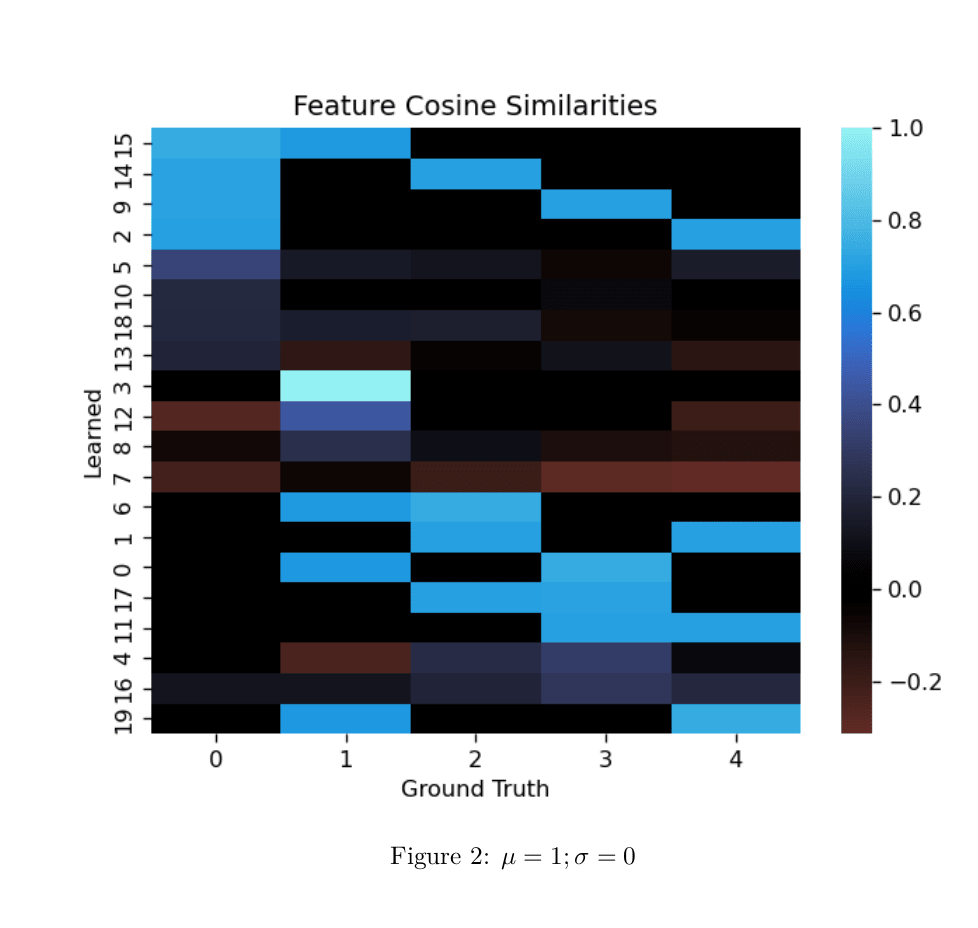
Edit: Remembered I have a larger example of the phenomena. Same setup as above.
Thank you!
That's super cool you've been doing something similar. I'm curious to see what direction you went in. It seemed like there's a large space of possible things to do along these lines. DeepMind also did a similar but different thing here.
That's a great question, something I didn't note in here is that positive biases have no effect on the output of the SAE -- so, if the biases were to be mostly positive that would suggest this approach is missing something. I saved histograms of the biases during training, and they generally look to be mostly (80-99% of bias values I feel like?) negative. I expect the exact distributions vary a good bit depending on L1 coefficient though.
I'll post histograms here shortly. I also have the model weights so I can check in more detail or send you weights if you'd like either of those things.
On a related point, something I considered: since positive biases behave the same as zeros, why not use ProLU where the bias is negative and regular ReLU where the biases are positive? I tried this, and it seemed fine but it didn't seem to make a notable impact on performance. I expect there's some impact, but like a <5% change and I don't know in which direction, so I stuck with the simpler approach. Plus, anyways, most of the bias values tend to be negative.
I think you're asking whether it's better to use the STE gradient only on the bias term, since the mul (m) term already has a 'real gradient' defined. If I'm interpreting correctly, I'm pretty sure the answer is yes. I think I tried using the synthetic grads just for the bias term and found that performed significantly worse (I'm also pretty sure I tried the reverse just in case -- and that this did not work well either). I'm definitely confused on what exactly is going on with this. The derivation of these from the STE assumption is the closest thing I have to an explanation and then being like "and you want to derive both gradients from the same assumptions for some reason, so use the STE grads for m too." But this still feels pretty unsatisfying to me, especially when there's so many degrees of freedom in deriving STE grads:
Another note on the STE grads: I first found these gradients worked emperically, was pretty confused by this, spent a bunch of time trying to find an intuitive explanation for them plus trying and failing to find a similar-but-more-sensible thing that works better. Then one night I realized that those exact gradient come pretty nicely from these STE assumptions, and it's the best hypothesis I have for "why this works" but I still feel like I'm missing part of the picture.
I'd be curious if there are situations where the STE-style grads work well in a regular ReLU, but I expect not. I think it's more that there is slack in the optimization problem induced by being unable to optimize directly for L0. I think it might be just that the STE grads with L1 regularization point more in the direction of L0 minimization. I have a little analysis I did supporting this I'll add to the post when I get some time.